Taxonomy-invariant Object Recognition Evaluation (TORE)

Jun 11, 2026

Document layout analysis is a cornerstone of modern document AI pipelines. The task consists of locating and classifying the elements of a document. The location of each document element is described by a bounding polygon (e.g. bounding box) and a label is assigned to designate its class (e.g. Title, Table, Figure, etc.). The label is selected out of a taxonomy of pre-defined classes which is specific to the dataset or the model. Throughout this article we call the outcome of the layout analysis task for a single page as Layout Resolution. Essentially the layout resolution defines the location and label for the detected elements of one page.

Despite the importance of layout analysis for document understanding, evaluating how well a model performs this task turns out to be surprisingly tricky. Three fundamental difficulties stand out immediately:

The most widely used metric, mean Average Precision (mAP), is known to have many limitations that make it inappropriate for evaluating the layout analysis of documents.
Most evaluation methods only apply when both the reference layout resolution and the resolution under evaluation use the same class taxonomy. This excludes cases such as:
- Evaluating a model on a dataset with annotations that use a different taxonomy.
- Comparing directly two models against each other, where each model uses its own taxonomy.
We want an efficient implementation that utilizes the capabilities of a modern CPU for parallelism and Single Instruction Multiple Data (SIMD) operations.

In this article we will present the "Taxonomy-invariant Object Recognition Evaluation (TORE)" method, which overcomes all of the above limitations.

TORE has been open sourced as part of the docling-metrics package and it is essential part of the Docling project.

1. Evaluation Challenges in Layout Analysis

As has already been observed [2], [5], [6], mean Average Precision suffers from several notable limitations. Most critically, mAP becomes meaningless when predictions lack confidence scores. Without a ranking mechanism, the Precision-Recall curve degenerates into a single point, rendering Average Precision nonsensical. However, many models provide predictions without confidence scores. Beyond this, mAP treats all predictions that meet the minimum IoU threshold as equally valid, regardless of how precisely they overlap with the ground truth. Implementation details such as PR curve interpolation, area computation methods, and caps on the number of predictions per image have also been shown to affect the evaluation results. Finally, mAP offers no diagnostic value: it provides no insight into which classes a model excels at or struggles with — information that would be invaluable during model development.

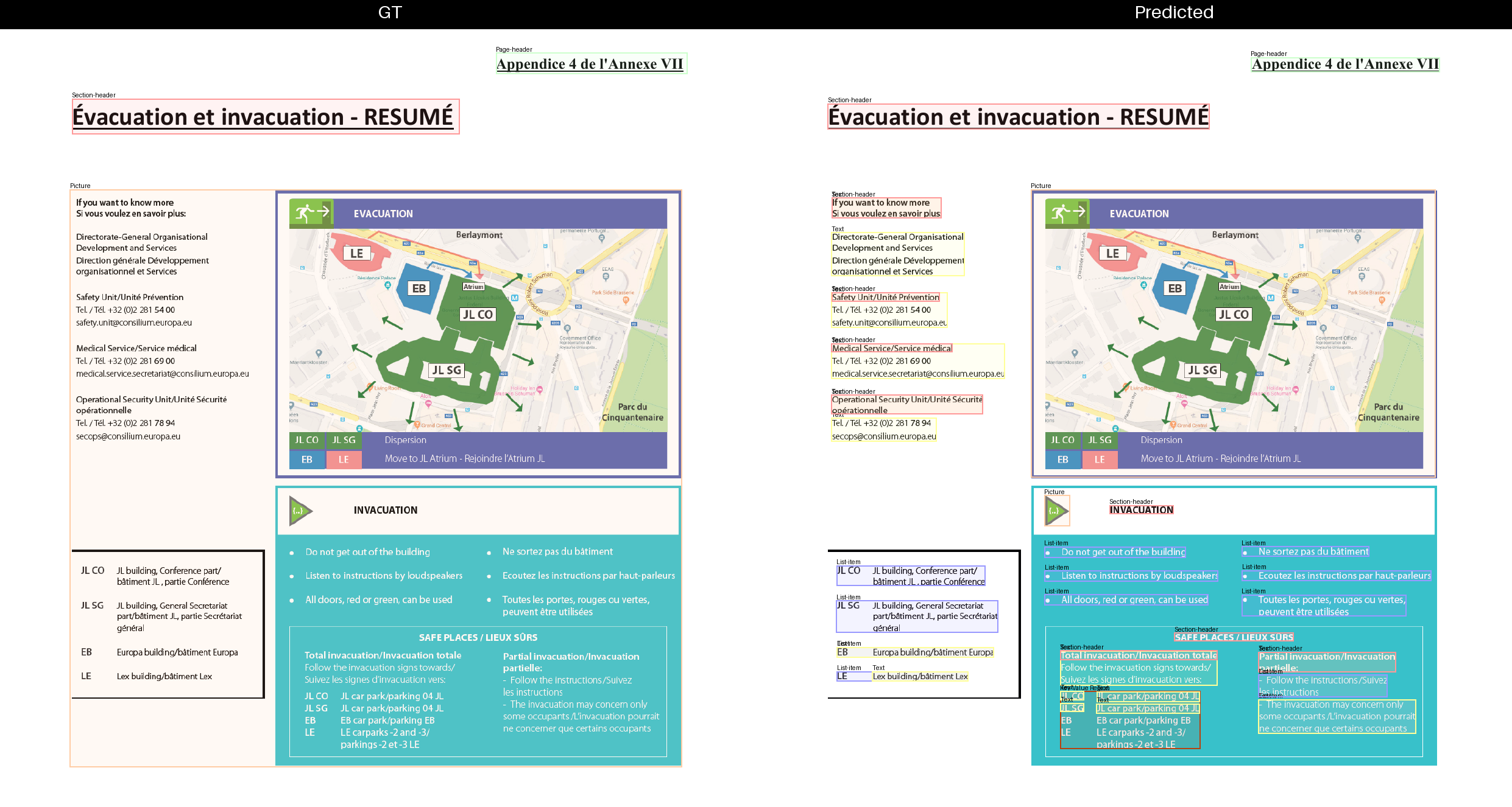
A qualitative study of layout analysis in real-world documents, reveals that the high complexity of documents often yields ambiguous annotations. As shown in Figure 1, it is not clear whether the ground-truth data (left) or the model predictions (right) are correct — or whether both are valid layout resolutions. In this example, the main body of the page is annotated as one large Picture. The model, however, predicts a more detailed layout: textual elements are identified as Section-Header, Text, and List-Item, and the picture bounding boxes are reduced to cover only the visual content.

Ambiguous predictions1 — *Figure 1. Ambiguous document layout analysis predictions.*

2. Single Taxonomy Confusion Matrix and its Derivatives

A confusion matrix is a tabular representation of a classifier’s predictions, where each row corresponds to the reference class (e.g. ground truth) and each column to the predicted class. The matrix cell c[i,j] denotes the number of samples belonging to class i that were predicted as class j. For a perfect classifier, the confusion matrix is diagonal. In real-life classifications, the diagonal entries quantify correct predictions and count as "Gains", while the off-diagonal entries correspond to mis-predictions and count as "Penalties".

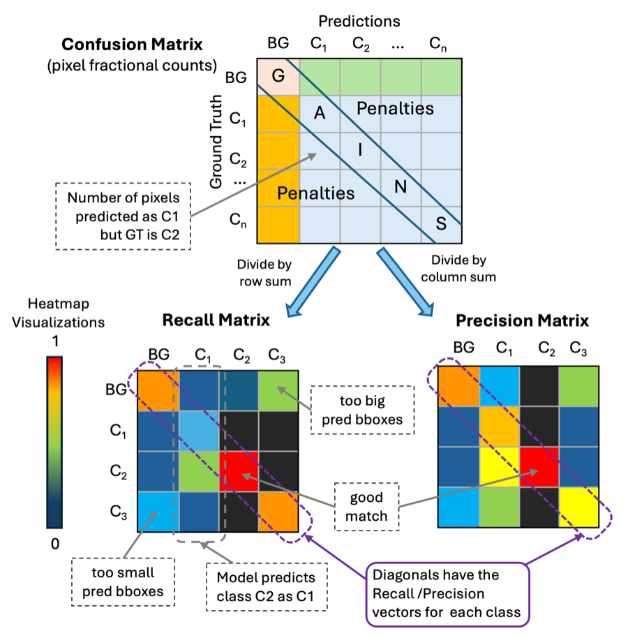
In Figure 2 we can see a Confusion Matrix built for the classes C1, C2, ... , Cn and the special Background class BG (in TORE each sample is a pixel of the rasterized layout resolution - more details below).

Several performance measures can be derived from the confusion matrix:

Recall matrix: A row-wise normalized confusion matrix, produced by dividing each cell over the sum of its row. The Recall Matrix provides a two dimensional break-down of the recall across the reference and predicted classes.
Precision matrix: A column-wise normalized confusion matrix, produced by dividing each cell over the sum of its column. The Precision Matrix provides a two dimensional break-down of the precision across the reference and predicted classes.
Recall and precision vectors: If we extract the diagonals of the corresponding Recall and Precision matrices we get the recall/precision values for each class individually.

Finally, the confusion matrix and its derived recall and precision matrices can be visualized effectively using heatmaps, enabling intuitive inspection of prediction patterns and systematic errors.

3. Building the Confusion Matrix

Document layout analysis is a multi-class and multi-label task.

In TORE we use the approach described in the paper [4] "Multi-Label Classifier Performance Evaluation with Confusion Matrix". The main idea is the "Algorithm 1" listed on page 9, which distinguishes 4 cases and assigns fractional "Gains" and "Penalties" for each sample of the dataset. The 4 cases are:

Case 1: The classifier has assigned to the sample the same label as in ground-truth (perfect match).
Case 2: The classifier has assigned to the sample the label of the ground-truth plus some additional wrong label(s) (over-prediction).
Case 3: The classifier has assigned to the sample only a subset of the ground-truth labels (under-prediction).
Case 4: Predicted and ground-truth labels have some partial overlap and some diff (diff-prediction).

TORE computes the Confusion Matrix and its Recall/Precision matrices for a collection of documents as follows:

Rasterize the layout resolution both for the "reference" and the predictions:
- Each resolution is projected on top of the input page.
- As a result, the rasterized pixels corresponding to annotations/detections are assigned one or more labels.
- Multiple labels for the same pixel may occur due to overlapping predictions.
- Assign the special class Background to the pixels without any annotations/detections.
- The "reference" resolution can be either ground-truth annotations or detections of a "reference" model.
Compute the confusion matrix and its derivatives Recall- and Precision Matrix using Algorithm 1 for each page:
- Each rasterized pixel becomes a sample input for Algorithm 1.
- Notice: The "Case 3" of Algorithm 1 never happens when we have single label annotations/predictions.
Sum up the matrices of each page to produce the ones at the dataset level.

4. Example 1: TORE with a Single Taxonomy

In the next example we will show what the confusion, recall and precision matrices look like when we apply the TORE metric on the "Heron" model for document layout analysis [2], [3].

The "Heron" model uses a taxonomy of 17 classes:

[
    "Caption", "Footnote", "Formula", "List-item", "Page-footer", "Page-header", "Picture",
    "Section-header", "Table", "Text", "Title", "Document Index", "Code",
    "Checkbox-Selected", "Checkbox-Unselected", "Form", "Key-Value Region"
]

Figure 3 shows the "Confusion Matrix" of the model against the DocLayNet-v2 dataset, which uses the same class taxonomy. Additionally, the class Background has been added as the first row/column. The rows correspond to the ground-truth, the columns to the predictions and each cell(i,j) shows the number of pixels that belong to class-i but have been predicted as class-j. Notice that the pixel counts are fractional, due to the way "Algorithm 1" distributes "Gains" and "Penalties". We use a color code to indicate the magnitude of the cell counts and highlight the main diagonal with pink border.

Heron - Confusion Matrix — *Figure 3. The Confusion Matrix of Heron model on the DocLayNet v2 dataset*

In Figure 4 we can see the Recall matrix. Remember that a perfect classifier should have red cells on the diagonal and black elsewhere.

As we can see in the example of "Heron" the recall matrix provides significant insight into the performance of the model. We can immediately see for which classes the model performs well, and, in case of mis-classifications, which classes the model confuses. For example we can see that "Heron" performs excellently on Background and quite well for the classes: Picture, Table, Text, Document Index, Code and Form. The recall for Checkbox-Selected and Checkbox-Unselected is still high but a bit lower. The model lacks recall mostly for the classes Key-Value Region and Title. Also the recall reveals that "Heron" tends to mis-classify Title as Section-Header.

If we extract the cells of the main diagonal we get the Recall Vector.

Heron - Recall Matrix — *Figure 4. The Recall Matrix of Heron model on the DocLayNet v2 dataset*

In Figure 5 we can see the Precision Matrix. The precision matrix can also help to derive interesting conclusions about the performance of a model. For example we see a high off-diagonal value for the cell [Background, Key-Value Region], which indicates that Heron misses key-value bounding boxes and mis-classifies them as Background.

If we extract the cells of the main diagonal we get the Precision Vector.

Heron - Precision Matrix — *Figure 5. The Precision Matrix of Heron model on the DocLayNet v2 dataset*

5. Reduced Matrices

As we saw in the previous sections the Confusion, Recall and Precision matrices are an invaluable source of information. At the same time, this information can be overwhelming. In Heron's case, it means analyzing three 18x18 matrices. One way to condense this information is to sum the cell values of all non-background classes into one class. This way we produce reduced 2x2 matrices for the Background class and the non-Background super-class. This abstraction allows us to quickly check if the classifier can detect the elements of the page correctly, regardless of the type of document element.

For Heron, Figure 6 shows the reduced Recall and Precision matrices:

Heron - Reduced Recall & Precision Matrices — *Figure 6. Reduced Recall & Precision Matrices of Heron model on the DocLayNet v2 dataset*

6. Dual Taxonomies Confusion Matrix

So far we have built confusion matrices where both the reference (rows) and the predictions (columns) use the same classes. However, very often we need to compare model predictions against datasets or other models that use different class taxonomies. Assuming that the reference uses the classes BG, GT1, ..., GTn and the predictions use the classes BG, P1, ... , Pm, we can create a confusion matrix based on the union-taxonomy BG, GT1, ..., GTn, P1, ... Pm.

This extended matrix will be sparse and have the block structure shown in Figure 7 where the non-zero values are: - First column (Background) for the rows: [BG, GT1, ..., GTn] - Top left block, for the rows: [BG, GT1, ..., GTn] and columns: [BG, P1, ..., Pm].

All other values are zero as the model never predicts on the reference taxonomy and the evaluation is never done against the prediction's taxonomy.

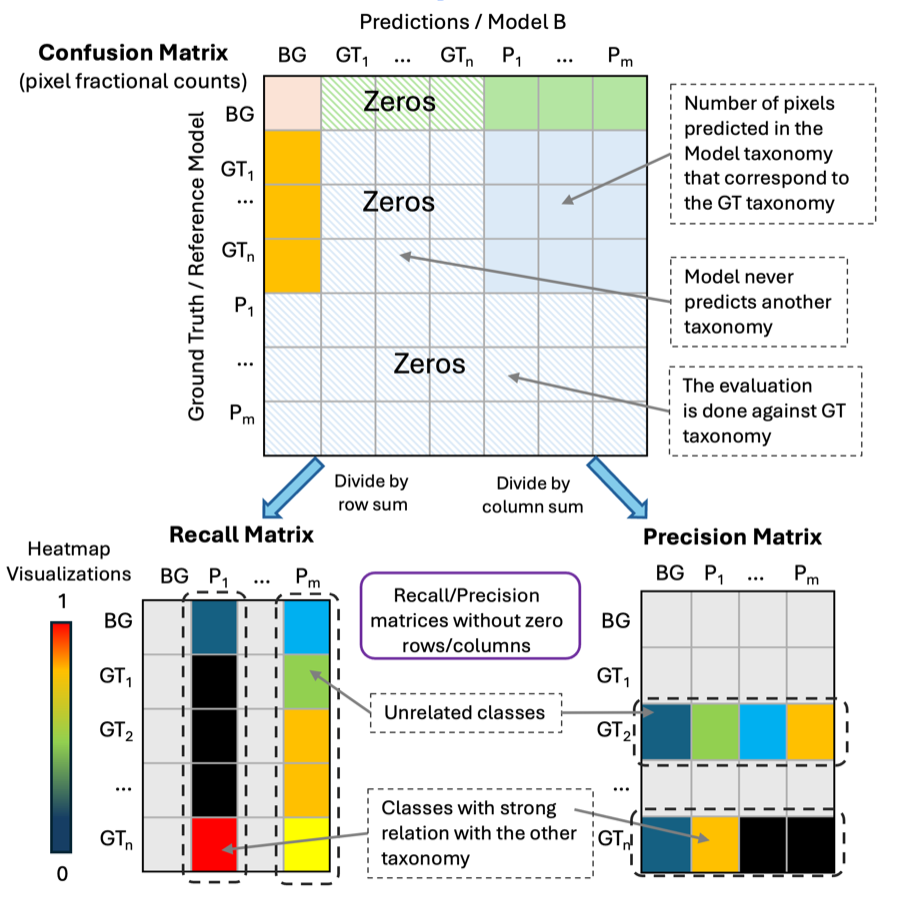
Dual taxonomy confusion matrix — *Figure 7. Dual class taxonomies matrices*

As shown in Figure 7 we can derive the Recall and Precision matrices by dividing each value by its row/column sum. Notice that the classic recall and precision vectors per class can no longer be computed, as the diagonals of the recall and precision matrices are no longer meaningful.

What can be extracted, however, is highly informative. Reading the Recall Matrix row-by-row reveals how each reference class maps to the prediction classes. A "bright" column (many large values) flags a prediction class that systematically absorbs many reference classes — the classifier's "default" choice when it cannot assign the proper class.

Conversely, reading the Precision Matrix column-by-column reveals how each prediction class maps to the reference classes. A "bright" row indicates a reference class that suffers "systematic leakage", with many prediction classes mapping into it.

Additionally, similarly to what happens with the same class taxonomy matrices, it is possible to reduce the matrix by collapsing all non-background classes into one class.

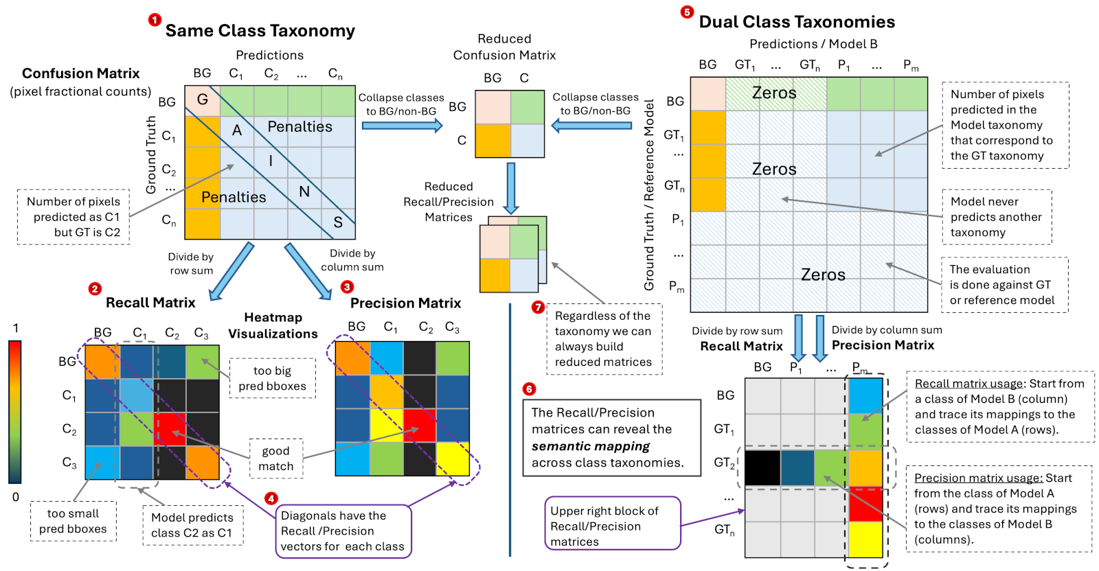
Figure 8 shows the full picture for the same class taxonomy and dual class taxonomies confusion matrices and their derivatives.

Multiple taxonomies matrices — *Figure 8. Multiple class taxonomies matrices (read the diagram in the indicated order)*

7. Example 2: TORE with Dual Taxonomies

In this example we want to demonstrate how TORE can be used to compare models with different class taxonomies. We will use "Heron" as the reference and compare it to "nemotron-page-elements-v3". The "nemotron-page-elements-v3" model uses the following class taxonomy:

["table", "chart", "title", "infographic", "text", "header_footer"]

The input pages are taken from the test split of the "ViDoRe V3" dataset. Notice that in this example we do not compare the models against any ground truth, but against each other. We have selected "Heron" as the reference and "nemotron-page-elements-v3" as the measured model, but it could be the other way around.

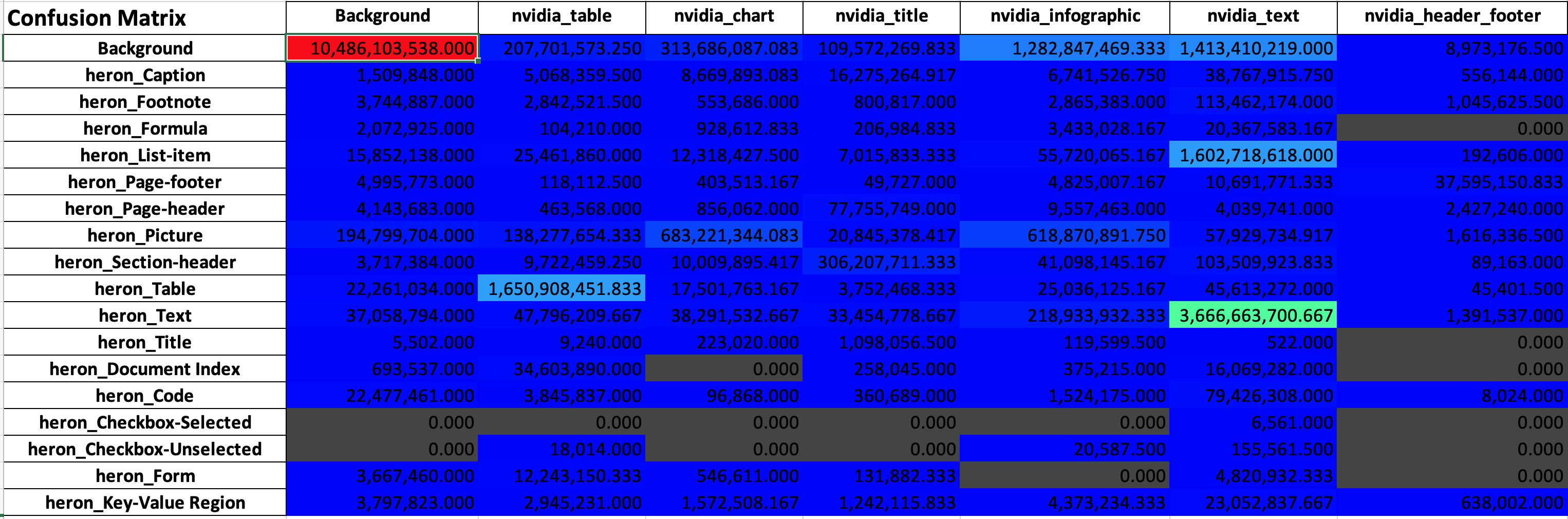
In Figure 9 we illustrate the full dual-taxonomy Confusion Matrix (click on the Figure to zoom in). The matrix has the expected block shape as described in Section 6, with the following all-zero regions:

The columns corresponding to the classes of the reference model ("Heron"). This happens because the measured model "nemotron-page-elements-v3" is never going to predict the classes of "Heron".
The rows corresponding to the classes of the measured model ("nemotron-page-elements-v3"). This happens because the evaluation is done only for the classes of the reference model ("Heron").

Heron - nemotron - Full Confusion Matrix — *Figure 9. The full Confusion Matrix of Heron vs nemotron-page-elements-v3 over the ViDoRe V3 dataset*

In order to improve the readability, we have redrawn the confusion matrix while hiding the all-zeros rows and columns in Figure 10. This helps to focus on the non-zero cells and make some semantic comparison across the predictions of the two models.

Heron - nemotron - Confusion Matrix — *Figure 10. The Confusion Matrix of Heron vs nemotron-page-elements-v3 without the zero rows/columns*

Similarly we provide illustrations of the Recall and Precision matrices while hiding the all-zero rows/columns in Figures 11 and 12 respectively.

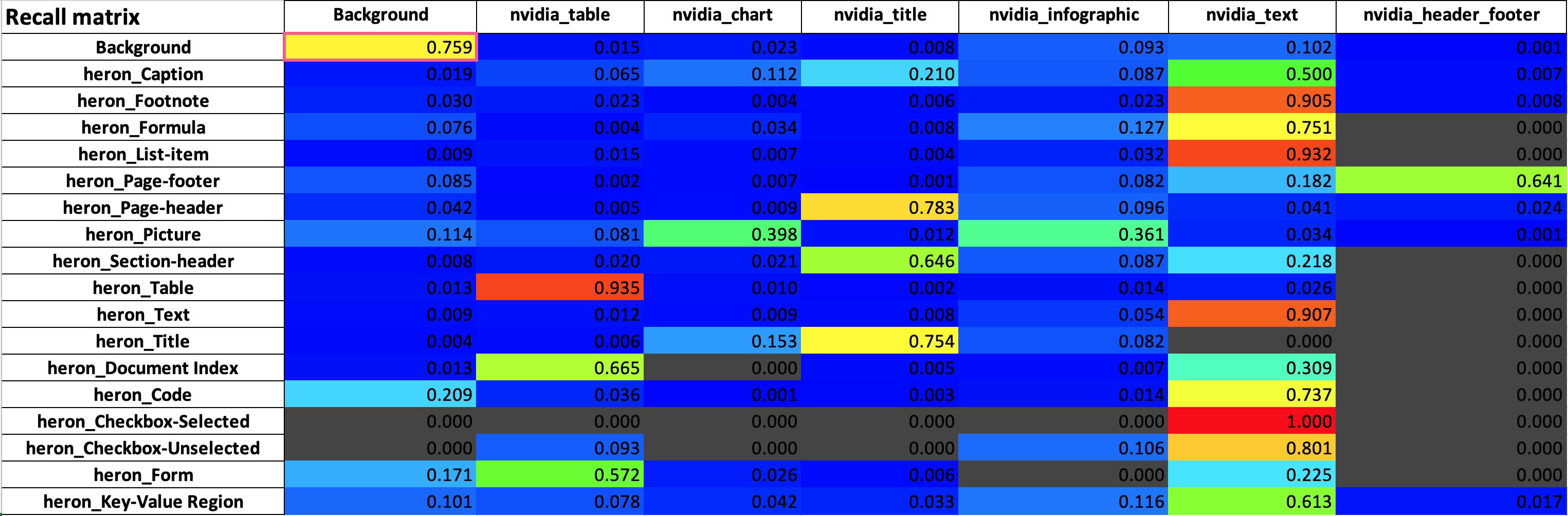
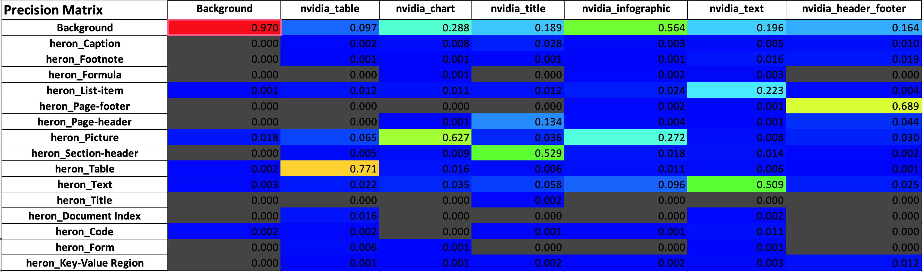
Heron - nemotron - Recall Matrix — *Figure 11. The Recall Matrix of Heron vs nemotron-page-elements-v3 over ViDoRe V3*

Heron - nemotron - Precision Matrix — *Figure 12. The Precision Matrix of Heron vs nemotron-page-elements-v3 over ViDoRe V3*

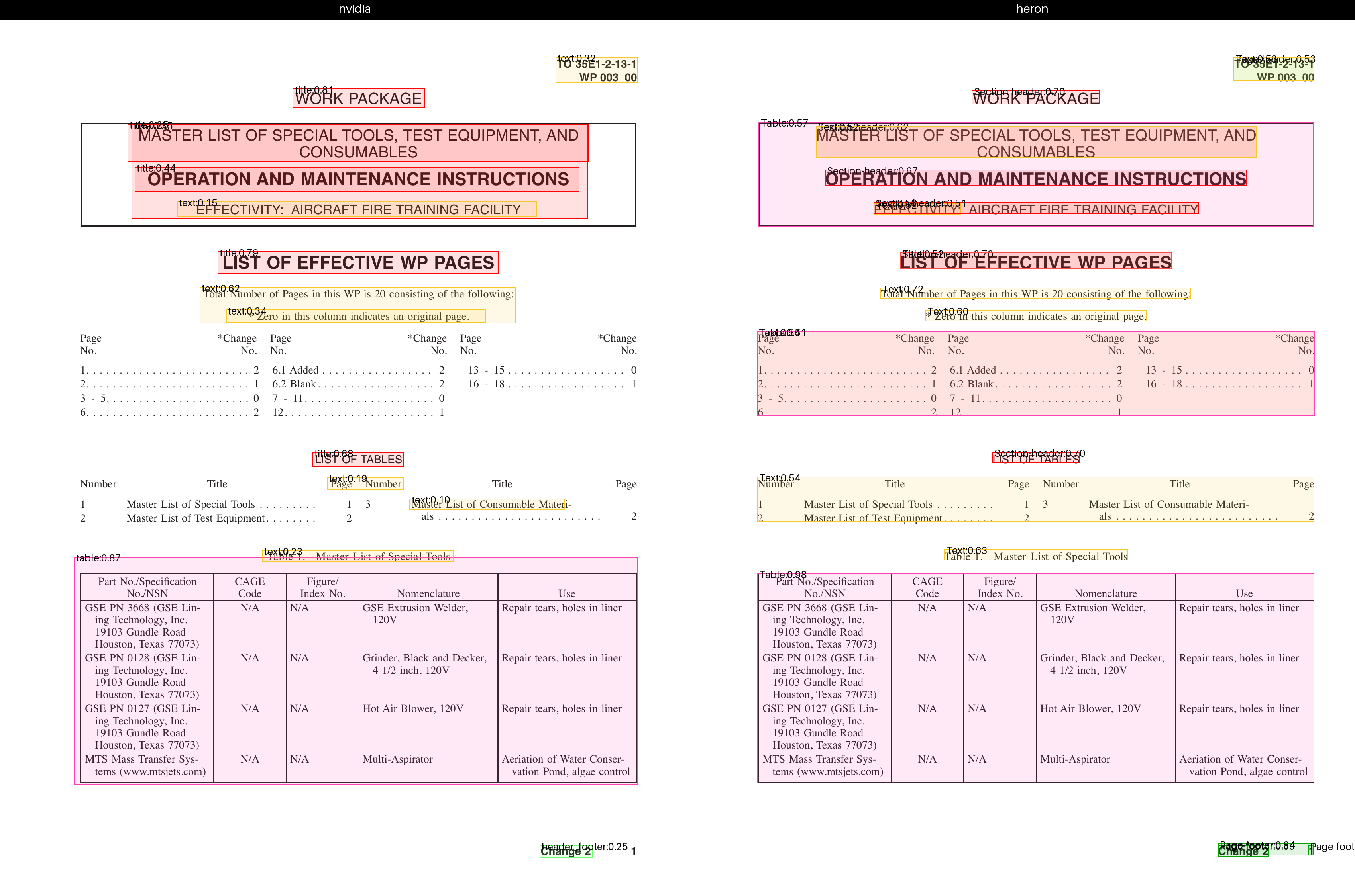
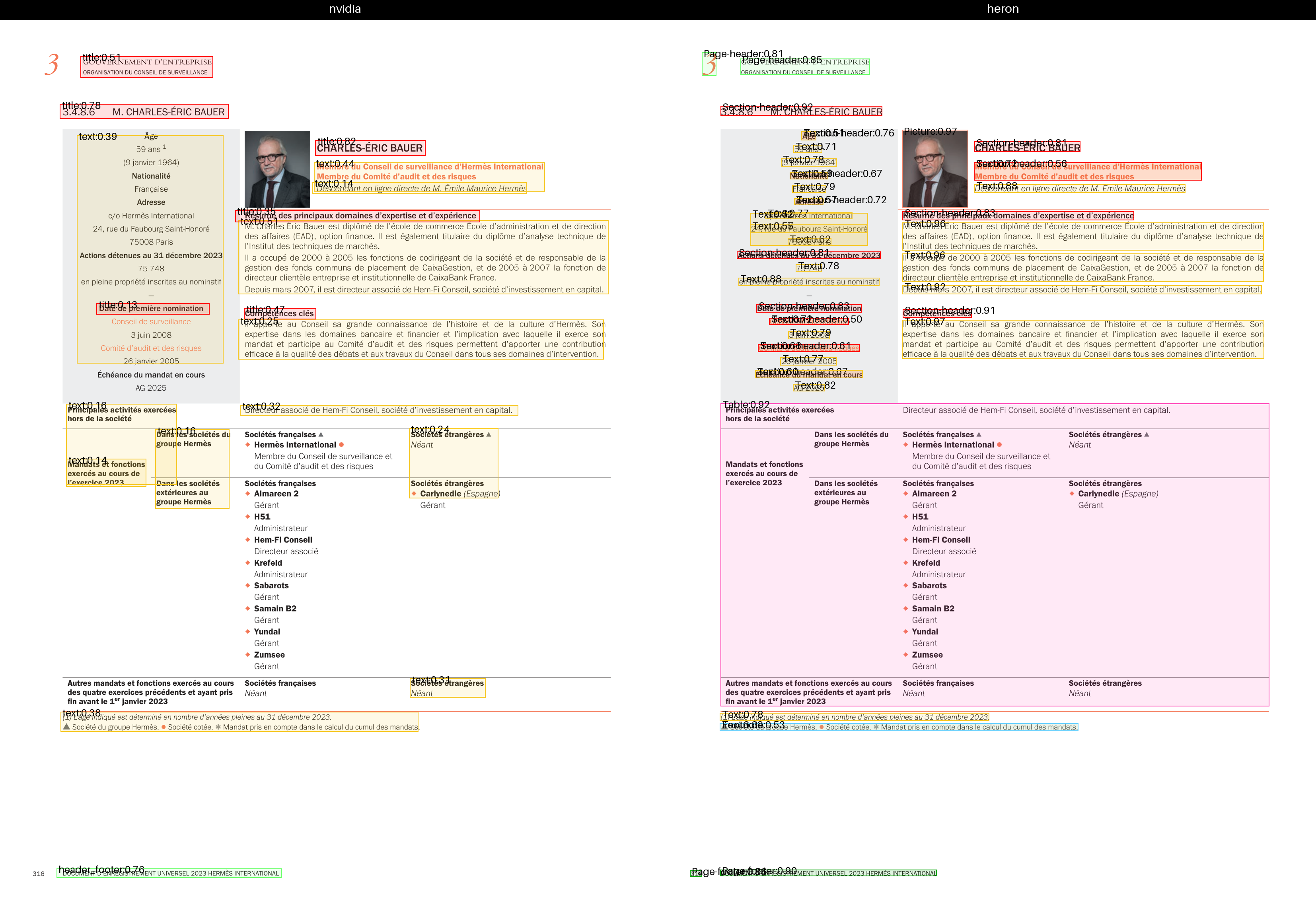
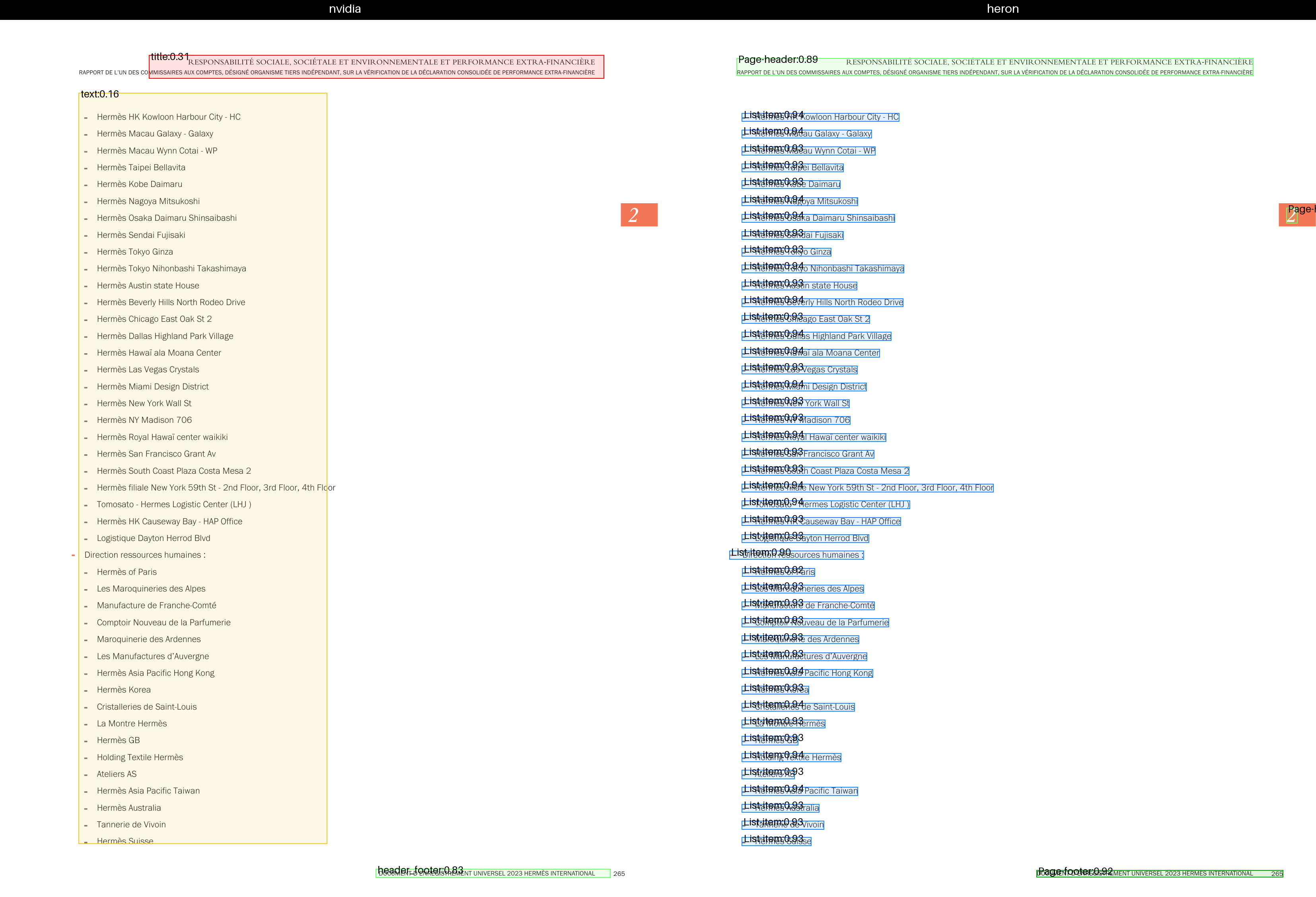
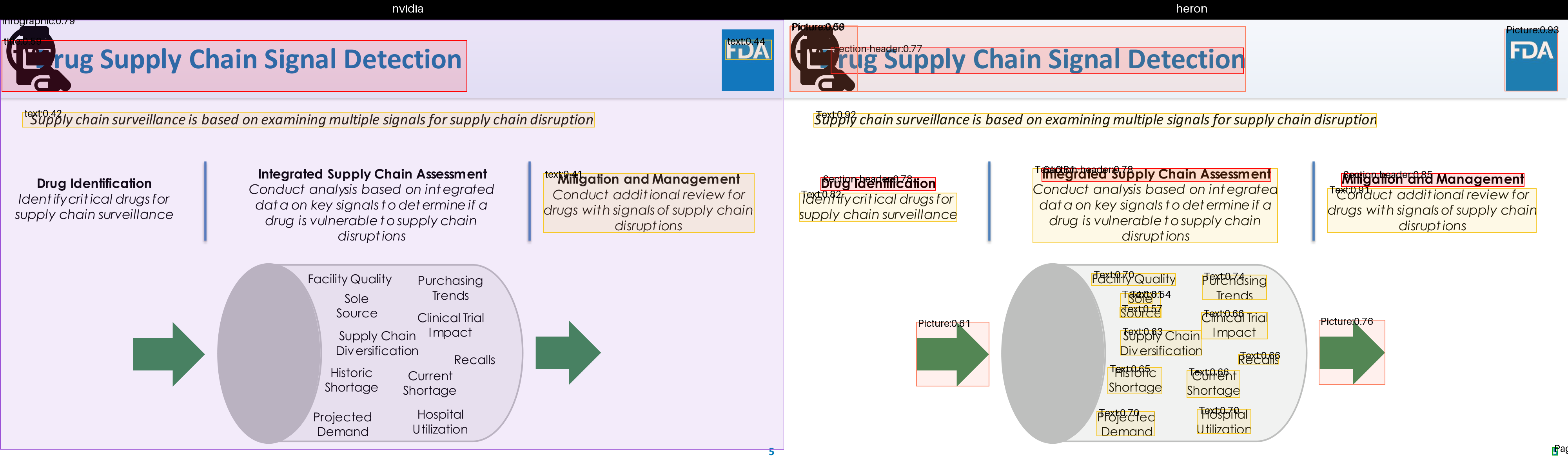
We can use the Recall and Precision matrices to gain insight into how the two models' predictions compare to each other. Additionally, visualizations of the predictions from selected pages can help to see in practice the differences in the behavior of the two models (see Figures 13, 14, 15, 16). All pages are taken from the ViDoRe V3 dataset and the actual doc_id and page_no are shown in the figure caption. On the left side are the predictions of Nvidia's "nemotron-page-elements-v3" and on the right side is "Heron".

First we can examine the Recall matrix row-by-row and see how the Heron classes map to Nemotron based on their semantic similarity. Here are some interesting observations:

Very strong similarity: heron_Table almost always maps to its semantic counterpart nvidia_table. The example in Figure 13 shows such a case.
Strong similarity: heron_Page-header maps 78% of the samples to nvidia-title. All examples in Figures 13-16 demonstrate such cases.
Weak similarity: heron_Section-header maps to nvidia_title in 64% of the cases and to nvidia_text in 21% of the cases. Similarly heron_Document Index and heron_Form map around 2/3 of the cases to nvidia_table and 30% - 20% to nvidia_text. Also the heron_Picture maps equaly to nvidia_chart and to nvidia_infographic. The example in Figure 16 demonstrates this case.
Very week similarity: A wide range of Heron classes (heron_Caption, heron_Footnote, heron_Formula, heron_List-Item, heron_Text, heron_Code, heron_Checkbox-Selected, heron_Checkbox-Unselected, heron_Key-Value Region) map to nvidia_text. This is a very strong indication that Nemotron uses its "text" class as the "default" class for many Heron classes. However this is expected given that Nemotron has a much narrower taxonomy than Heron (6 vs 17 classes) and the broad scope of the "Text" class. Nemotron has simply no better class to map all those Heron classes but use its Text class.

Moving to the Precicion matrix, we can inspect it column-by-column and see how the Nemotron classes map to the Heron classes. For this matrix the semantic mapping is more evident as we examine it in the direction from the more generic (Nemotron's taxonomy) to the more specific (Heron's taxonomy).

Very strong similarity: nvidia_table maps mostly to heron_Table, nvidia_header_footer mainly to heron_Page-footer and nvidia_text maps strongly to heron_Text. The example in Figure 15 shows how both models correctly identified the page footer using their corresponding classes.
Outliers: The nvidia_title class maps in 52% of the cases to heron_Section-header despite the fact that the heron_Title class exists too. Also the class nvidia_text maps 22% of the cases to heron_List-item. This is an indication that the Nemotron model is not trained to distinguish "section header" and "list" document elements. Figure 15 demonstrates a characteristic case where a list is classified as text by Nemotron and List-Item by Heron.
Leakage to the Background: We notice that almost all non-background Nemotron classes map to heron's Background class. This indicates that Nemotron produces too large bounding boxes that leak into the background of the page. This can be easily confirmed by checking actual prediction samples like the one shown in Figure 16, where a single Infographic box covers the entire page. On the other hand Heron tends to detect the position of the document elements more accurately.

Heron vs nemotron example — *Figure 13. Nemotron vs Heron: Example1 (doc_id=viz_AFD-100607-009, page_no=22)*

*Figure 13. Nemotron vs Heron: Example1 (doc_id=viz_AFD-100607-009, page_no=22)*

*Figure 14. Nemotron vs Heron: Example2 (doc_id=viz_hermes_2023, page_no=320)*

*Figure 15. Nemotron vs Heron: Example 3 (doc_id=viz_hermes_2023, page_no=269)*

*Figure 16. Nemotron vs Heron: Example 4 (doc_id=viz_State_of_CDER_FDLI2021_PCavazzoni_20210515, page_no=4)*

8. Implementation Optimizations

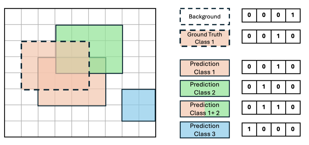
As already mentioned, the first step in TORE is to project the document layout resolution on the image pixels. This process happens both for the reference resolutions and the predictions. In the TORE implementation we bit-pack up to 64 labels per pixel inside an unsigned 64-bit integer (uint64). In our encoding we allocate the index-0 to the BG class and support up to 63 additional labels per pixel, which provides enough space for overlapping bounding boxes. This dense representation enables an efficient implementation of the TORE algorithm, which computes multiple pixels in parallel using SIMD operations via the NumPy library.

Figure 17 provides an example of the binary representation for the pixel labels used in TORE.

After rasterization, a compression step further reduces the computational cost. Instead of processing every pixel independently, the implementation counts the number of distinct pixel-pairs [reference, prediction] that appear on the page. The contribution matrix of each unique pair is computed only once and then multiplied by the number of times this pair appears. Because the number of unique pixel-pairs is substantially smaller than the total pixel count, this dramatically reduces the computational overhead. Finally we parallelize the computation of the page-level confusion matrices.

TORE Binary Representation — Figure 17. Example of TORE binary representation using uint4 (TORE implementation uses uint64). The bboxes with dashed lines correspond to the reference resolution (e.g. ground-truth) and the solid ones to the predictions.

TORE has been open sourced as part of the docling-metrics package.

9. Summary

In this article we presented the "Taxonomy-invariant Object Recognition Evaluation" (TORE) metric and explained why it is well suited to evaluate the layout analysis of documents. We showed that the mean Average-Precision metric suffers from many limitations that make it unsuitable and even nonsensical when a model does not produce confidence scores. TORE overcomes these limitations through standard mathematical tools such as the confusion matrix and its derivatives, which provide not only evaluation measurements but also insights that help diagnose a model's mis-predictions.

One of TORE's major strengths is its ability to evaluate across heterogeneous classification taxonomies. This allows a model to be evaluated on a dataset that uses different classes, as well as direct model-to-model comparisons regardless of the underlying taxonomies. Via concrete examples we showcased how to use the confusion, recall and precision matrices and understand where the predictions of two models match and where they differ. Lastly we showed an efficient TORE implementation that accelerates the runtime performance of the metric via SIMD operations and parallelism.